
This project is a data analysis for a fictitious wealth management company called BlueSky Wealth Management. The analysis will mainly focus on the investments in fund by client for the organisation and the performance of these funds. As this is a fictitious organisation the data is not readily available hence I had to generate these using python. The analysis itself is done in SQL.
Tools Used


Overview
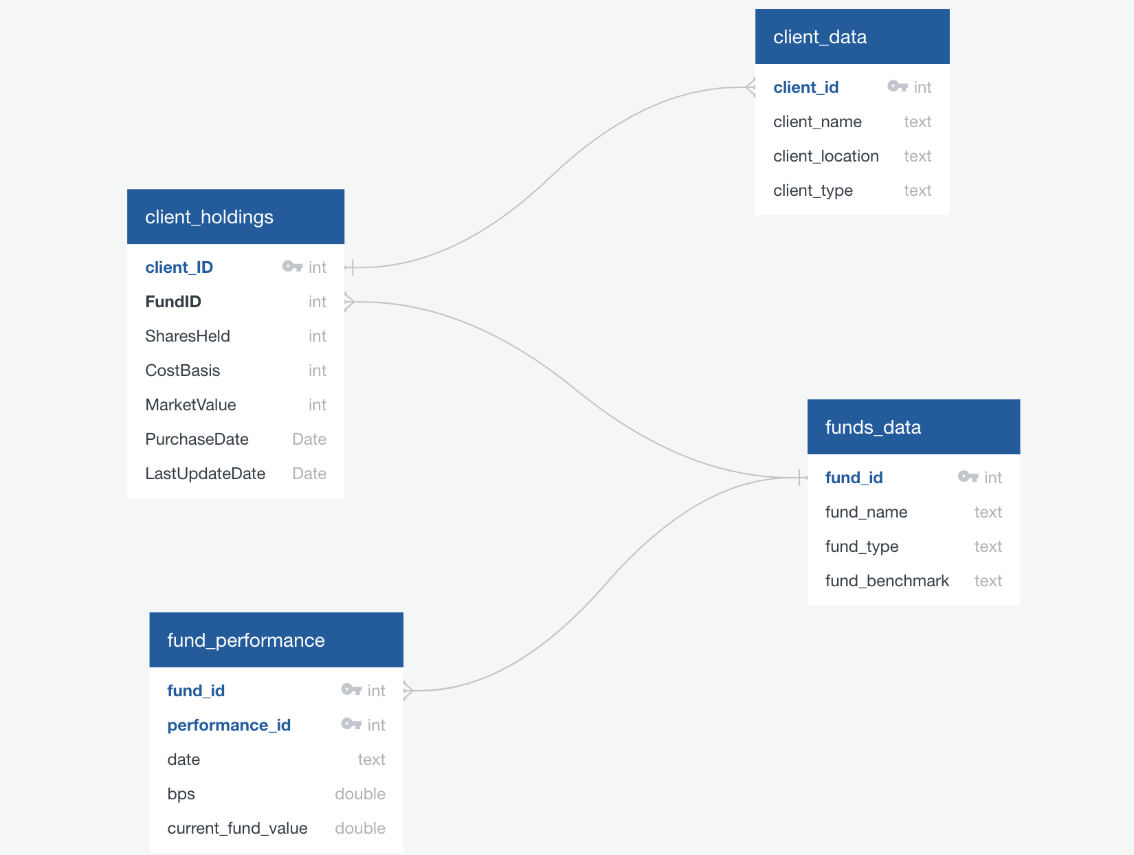
The database design for the database schema that stores information about clients and funds where developed in the four tables below:
client_data Table: This table stores information about clients, including their unique identifier (client_id), name (client_name), location (client_location), and type (client_type). The client_id is a primary key (PK) and can be used as a foreign key (FK).
client_holdings Table: The client_holdings table contains data related to the holdings of clients in the company’s portfolio. It includes columns for the client’s ID (client_ID), the fund’s ID (FundID), the number of shares held (SharesHeld), the cost basis of the holdings (CostBasis), the market value of the holdings (MarketValue), the date of purchase (PurchaseDate), and the last update date (LastUpdateDate).
fund_performance Table: This table is used to store data related to the performance of funds. It includes the unique identifier for the fund (performance_id which is a PK), a fund_id which is the foreign key to the fund data table, the date of the performance data (date), the basis points (BPS) , and the current fund value (current_fund_value).
funds_data Table: The funds_data table contains information about different funds, such as their unique identifier (fund_id, a PK), the fund’s name (fund_name), the fund type (fund_type), and the benchmark name (fund_benchmark). The fund_id can serve as an FK to establish a connection with the clients_funds_junction_tbl table.
Data Sets – Python
The data sets designed for the database above where created in python using a synthetic approach via “faker”. The below approach, was used to generate data and a data frame for the tables above. All output was generated into CSV file.
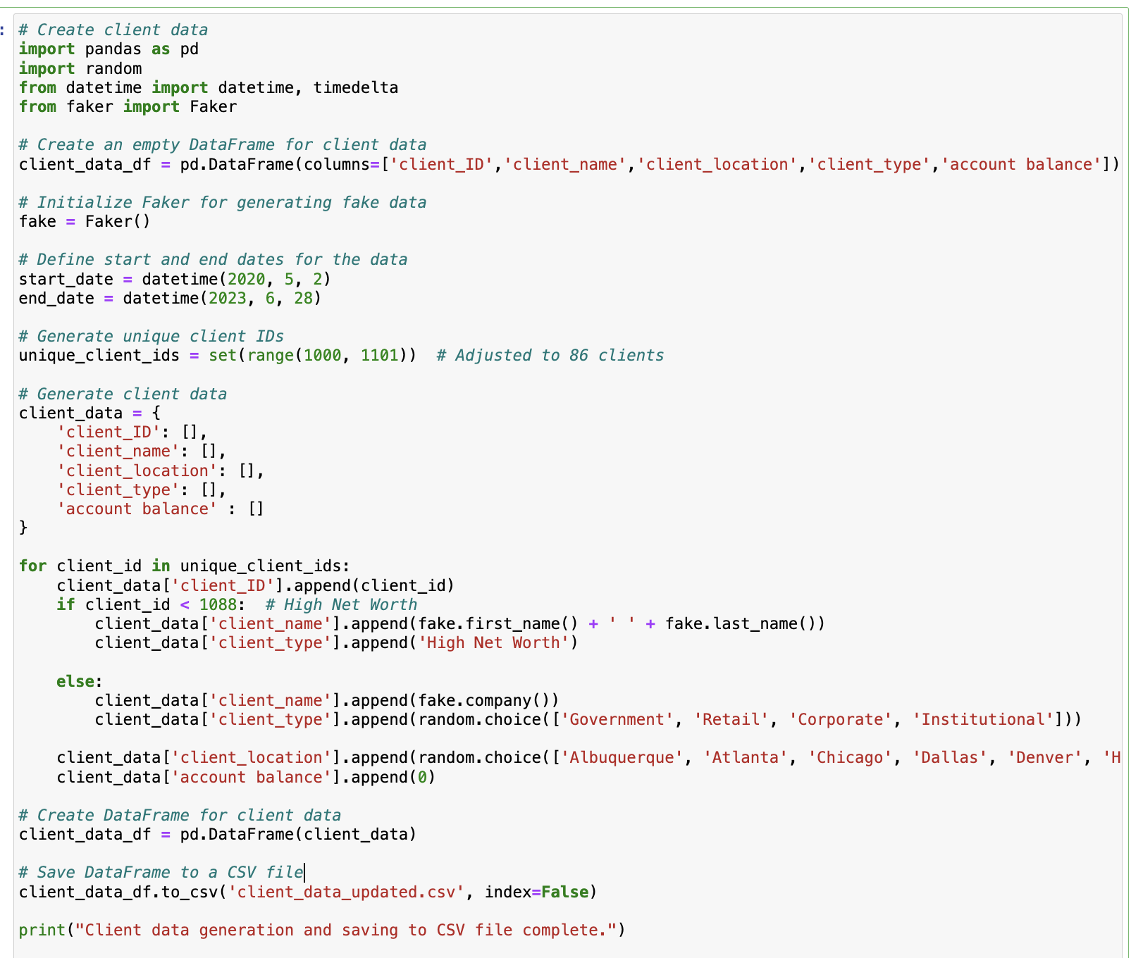
Client Data Generation:
This Python script creates synthetic client data for a portfolio. It generates information such as client names, locations, types, and account balances, and saves this data to a CSV file.
Fund Data Generation: The next script creates synthetic fund data. It generates unique fund IDs, fund types, fund names, fund managers, and benchmarks.
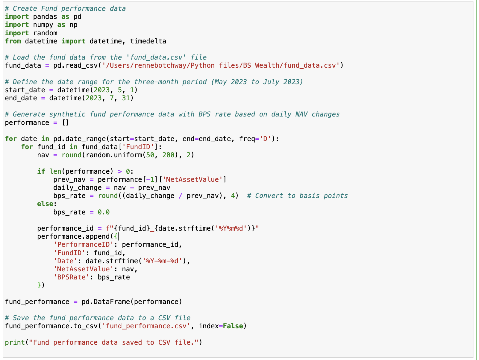
Fund Performance Data: This script loads the previously generated fund data and then creates synthetic fund performance data over a three-month period, from May 2023 to July 2023 (for sample purposes). The performance data includes the net asset value (NAV) and basis points (BPS) rate.
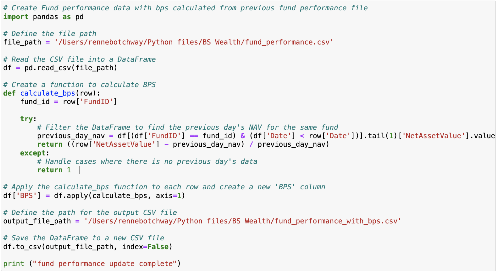
Fund Performance Data with BPS: In this script, BPS (basis points) is calculated for the fund performance data based on the previous day’s NAV.
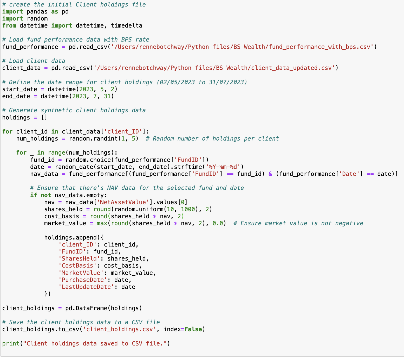
Client Holdings Data: This script generates synthetic client holdings data based on the previously created client and fund data. It simulates the number of holdings per client, fund IDs, shares held, cost basis, market value, and purchase dates.
Updated Client Holdings Data: In this final script, the client holdings data is updated for the bps rate calculation working out the daily change in NAV for each fund. The bps rate is useful as fund performance tracker.
SQL Queries
The data analysis for the “fake” data generated above in python is ow analysed using sql to gain some insight into the data generated and to ensure the logic applied is viable and correct.
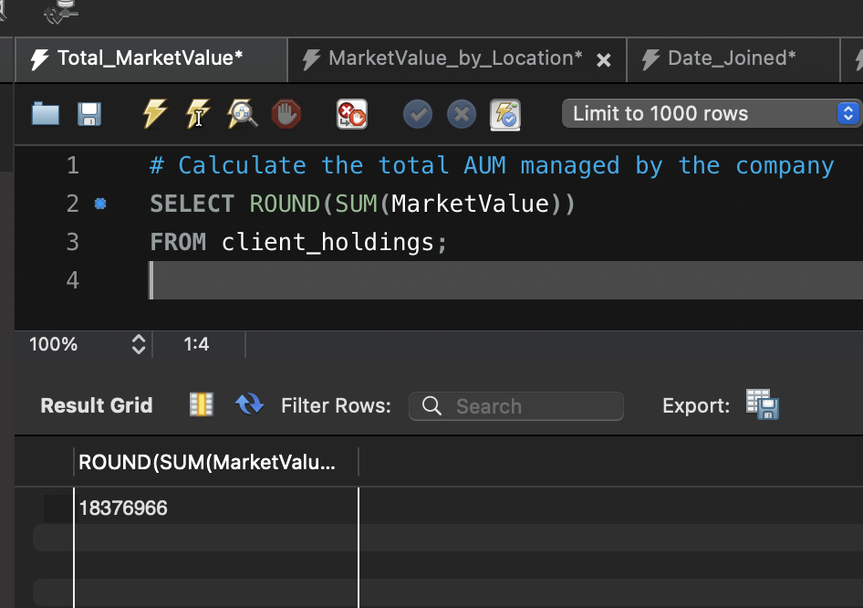
Query 1: Calculate the Total Assets Under Management (AUM) Managed by the Company
This SQL query calculates the total Assets Under Management (AUM) managed by the company. It does so by summing up the ‘MarketValue’ column from the ‘client_holdings’ table, which represents the market value of client holdings. The ROUND function is used to round the total AUM to the nearest whole number.
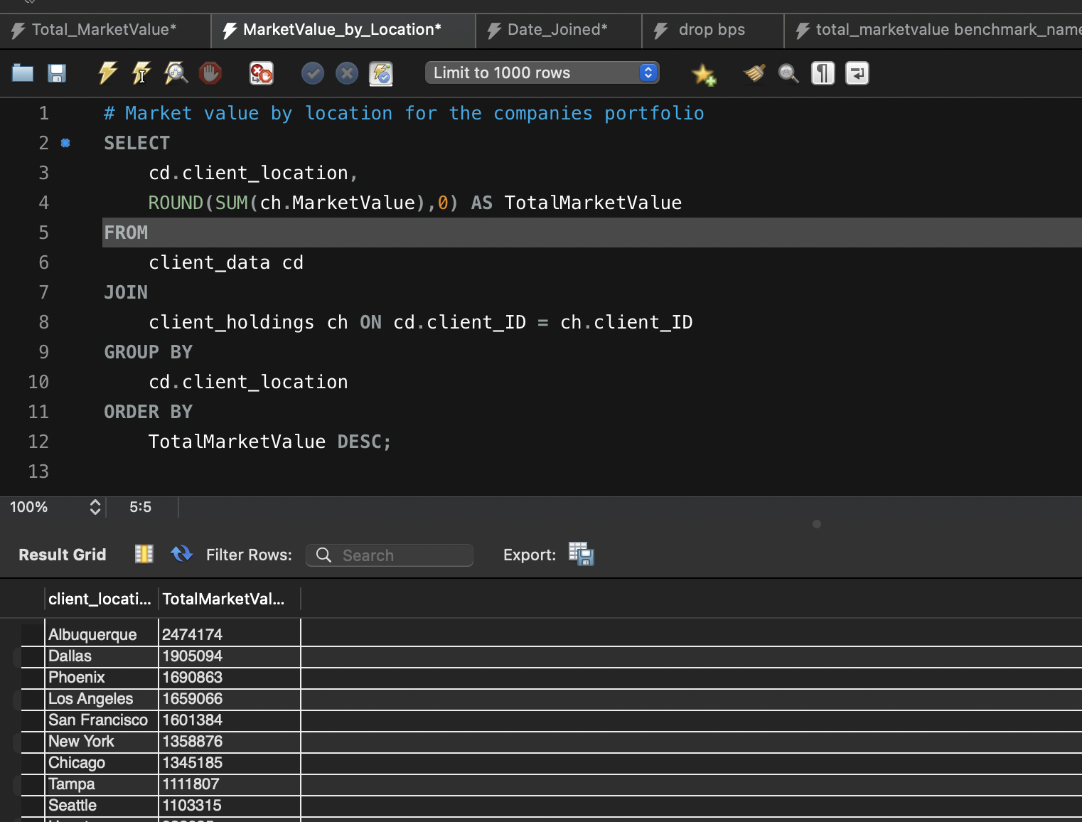
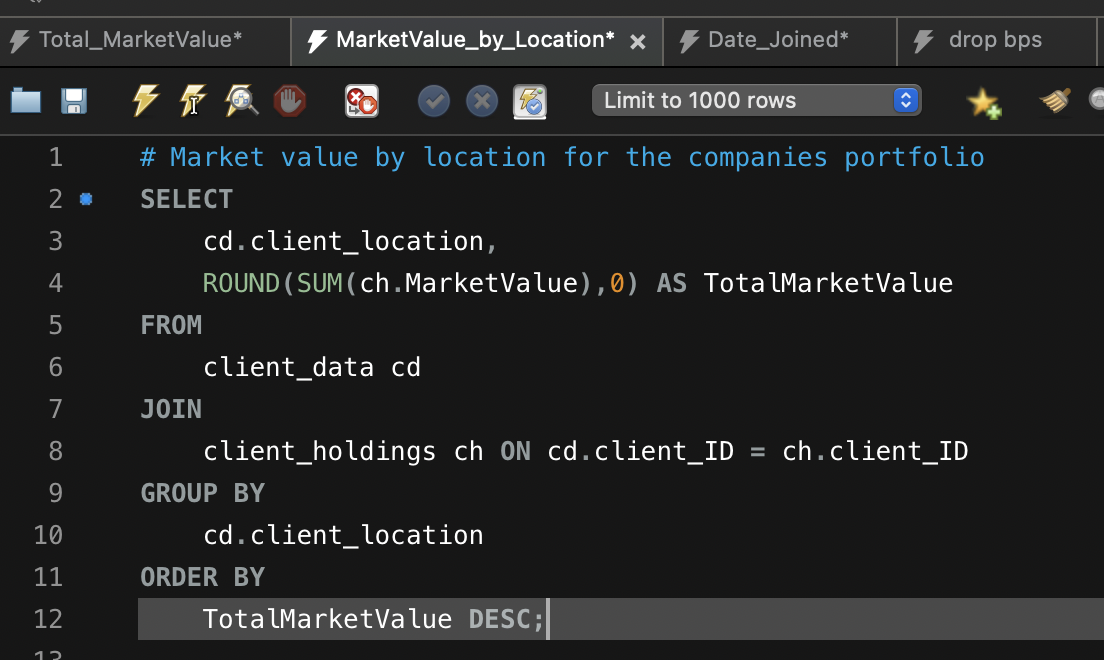
Query 2: Market Value by Location for the Company’s Portfolio
This query provides a breakdown of the total market value of the company’s portfolio by location. It retrieves data from both the ‘client_data’ and ‘client_holdings’ tables and groups the results by ‘client_location.’ The ROUND function rounds the ‘TotalMarketValue’ to the nearest whole number, and the results are ordered in descending order. This query helps visualise the distribution of assets by location.
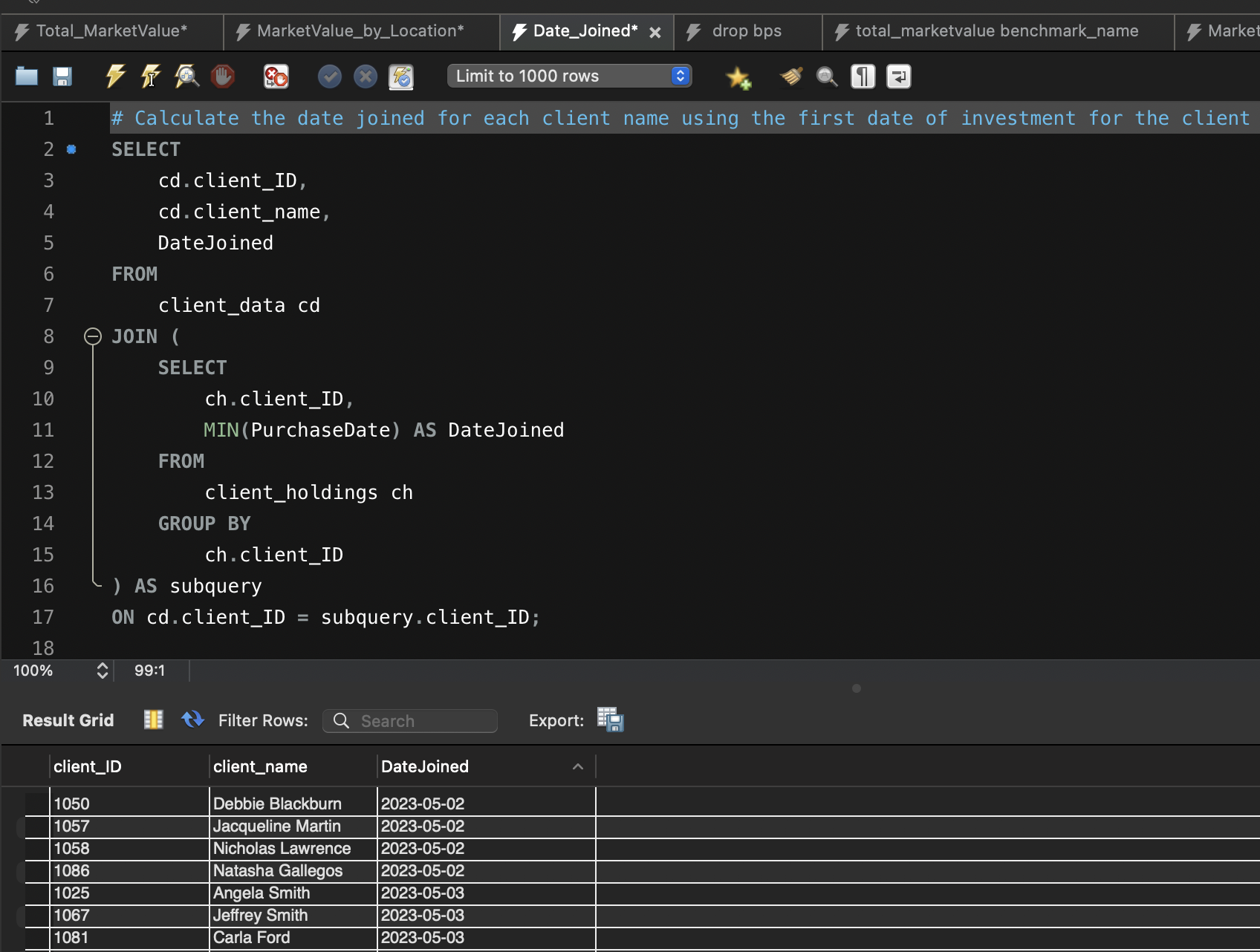
Query 3: Calculate the Date Joined for Each Client Name Using the First Date of Investment
This query calculates the date joined for each client by finding the earliest (minimum) ‘PurchaseDate’ from the ‘client_holdings’ table. It retrieves the client’s ID and name from the ‘client_data’ table and joins the results using a subquery. The subquery finds the minimum ‘PurchaseDate’ for each client. This information helps determine when each client became a part of the portfolio.
Query 4: Total Market Value by Benchmark Name
This query calculates the total market value for each benchmark used in the company’s portfolio. It combines data from the ‘fund_data’ and ‘client_holdings’ tables by matching ‘FundID.’ The ‘BenchmarkName’ and the rounded ‘TotalMarketValue’ are displayed for each benchmark. This analysis helps assess how different benchmarks contribute to the total portfolio value.
Query 5: Total Market Value for Each Client
Explanation: This query calculates the total market value for each client in the company’s portfolio. It retrieves the client’s name from the ‘client_data’ table and joins it with the ‘client_holdings’ table based on the client’s ID. The results are grouped by client name, and the ‘TotalMarketValue’ is rounded to the nearest whole number. This query provides insights into the value of each client’s holdings.
Data Visualisation
With all the data wrangling and integrity completed in sql the data in now connected to a visualisation tool in PowerBi.