Spark Internals, and What the Certification Does Not Cover

Notes on what Spark is actually doing when you call an action: the topology, the shuffle, the three optimisers, and how to read the evidence in the Spark UI. Built from screenshots I took while working through a Databricks project, and from the runs where something was clearly wrong and I had to go and find out why.

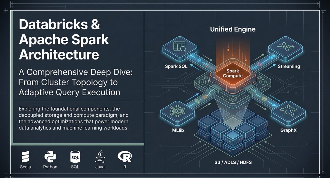
The thing to hold on to from that first picture is the separation. Spark is a compute engine that has been deliberately decoupled from storage, and the APIs on top of it are all lowered onto the same execution machinery. Whether you write SQL, PySpark or Scala, you end up in the same place. That is the reason the optimisations later in this post apply regardless of which one you use.

Part one: the machine

The physical topology

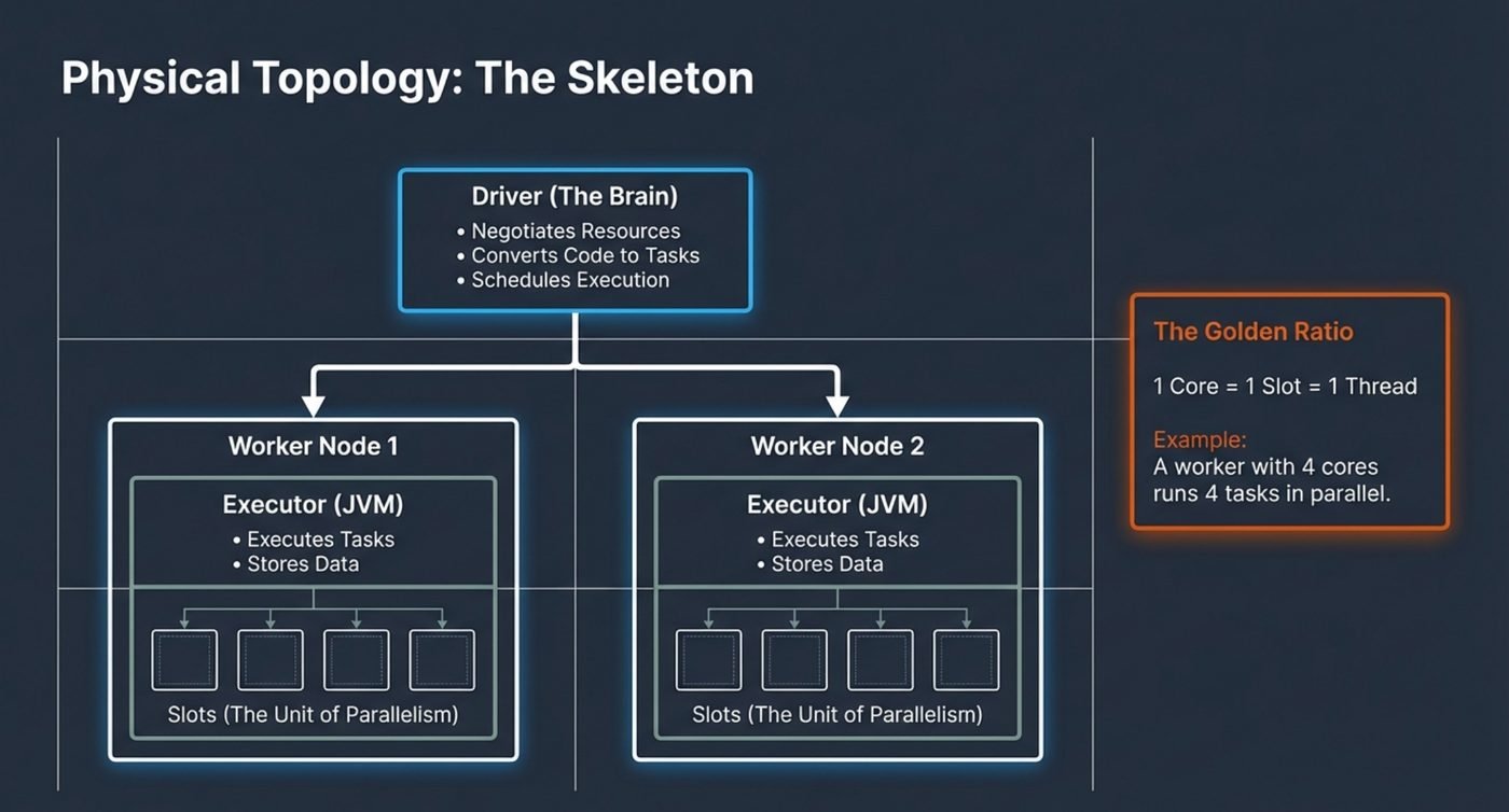
Three things matter here and everything else follows from them.

• The driver is the brain. It holds the plan, negotiates for resources, turns your code into tasks and schedules them. It is also a single point of contention, which is why collect() on a large DataFrame is a bad idea: you are asking every executor to ship its data to one JVM.
• The executor is a JVM on a worker node. It runs tasks and it stores data. Cached DataFrames live here, not on the driver.
• The slot is the unit of parallelism, and this is the ratio worth memorising: one core is one slot is one thread is one task at a time. A worker with four cores runs four tasks in parallel. Not five.

That last point is the arithmetic behind most cluster sizing arguments. If your job has 200 partitions and your cluster has 16 slots, you are running 13 waves of tasks. Adding executors helps until partitions divide evenly across slots, and then it stops helping.

The hierarchy of execution

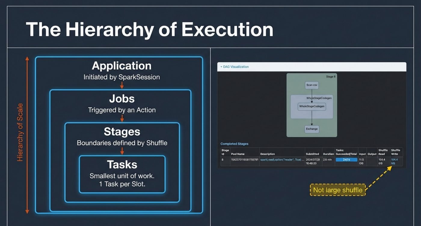
Four levels, and the useful part is what creates each boundary:

• An application is one SparkSession.
• A job is created by an action. One count(), one job.
• A stage is a run of work that can happen without moving data between executors. Stage boundaries are shuffles. If you want to know how many times your data crossed the network, count the stages.
• A task is one partition of data going through one stage on one slot.

Once you internalise that stages equal shuffles, the Spark UI stops being a wall of numbers. A job with two stages moved data once. A job with nine stages moved it eight times, and that is usually where the time went.

Part two: how Spark decides what to do

Laziness is the whole design

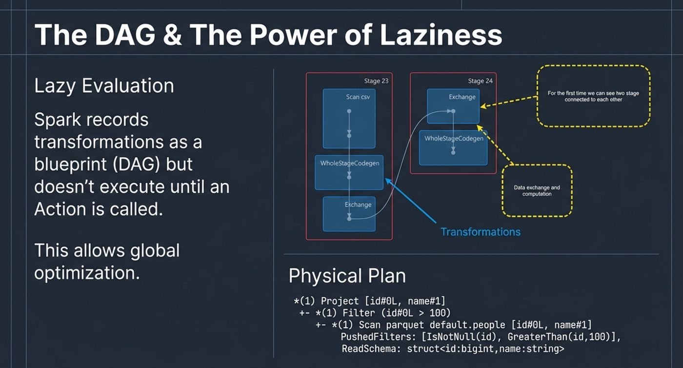
Nothing runs when you write it. Spark builds a directed acyclic graph of what you have asked for and waits. Only when an action arrives does it look at the whole graph and decide how to execute it.

This is not laziness for the sake of it. It is what makes global optimisation possible. Look at the physical plan in that screenshot:

*(1) Project [id#0L, name#1]
+- *(1) Filter (id#0L > 100)
   +- *(1) Scan parquet default.people [id#0L, name#1]
        PushedFilters: [IsNotNull(id), GreaterThan(id,100)],
        ReadSchema: struct<id:bigint,name:string>

The filter I wrote after the read has been pushed into the read. The scan will not return rows with id <= 100 at all, because Parquet can skip them at the row group level. Spark could only do that because it had not started executing when it saw the filter. Write the same logic eagerly, row by row, and that optimisation is impossible.

Transformations and actions

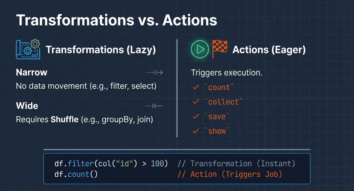
The distinction that actually predicts performance is not lazy against eager, it is narrow against wide.

• Narrow transformations like filter, select and withColumn can be done on each partition independently. No data moves. Spark will chain a whole run of them into a single stage and, as we will see with Tungsten, often into a single generated function.
• Wide transformations like groupBy, join, distinct and orderBy need rows that share a key to end up on the same executor. That means a shuffle, and a shuffle means a stage boundary.

When I am reviewing someone's Spark code, this is the first pass I make: how many wide transformations are in here, and does each one earn its place.

RDDs and DataFrames

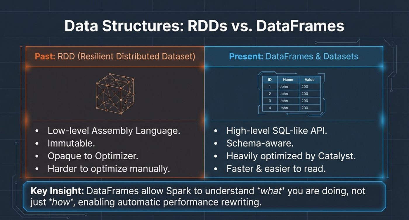
The framing on that slide is the right one. An RDD tells Spark how to do something. A DataFrame tells Spark what you want. Only the second one can be rewritten.

This is also the honest argument against Python UDFs. The moment you wrap logic in a Python function, Catalyst can no longer see inside it, so it cannot push it down, reorder it or fuse it. On top of that, rows have to be serialised out of the JVM into a Python worker and back. A UDF turns an optimisable declarative plan into an opaque box with a serialisation tax on both sides. If the same thing can be expressed with built in functions, it almost always should be.

Part three: where the time actually goes

The shuffle

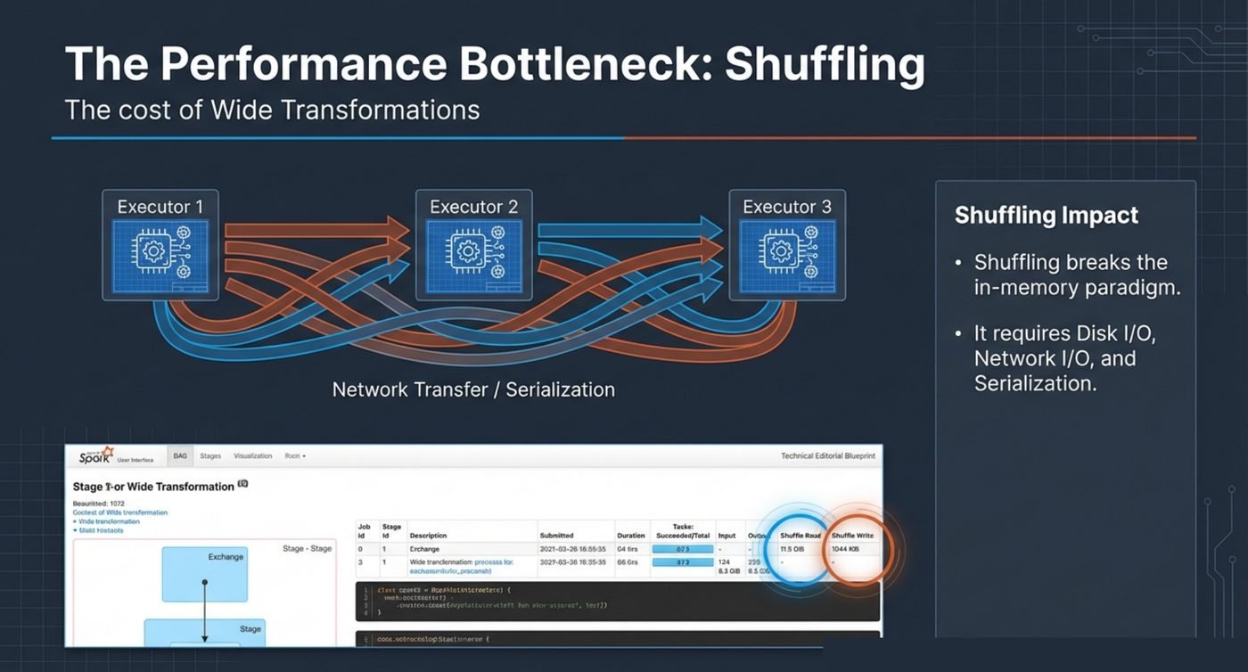
A shuffle is Spark writing intermediate data to local disk, then every executor reading the parts it needs across the network, deserialising them, and carrying on. Three expensive things at once: disk, network and serialisation.

Everything people say about Spark being an in-memory engine stops being true at a shuffle boundary. That is the moment it becomes a disk and network engine. Which is why the number of stages matters so much.

Cardinality decides how bad the shuffle is

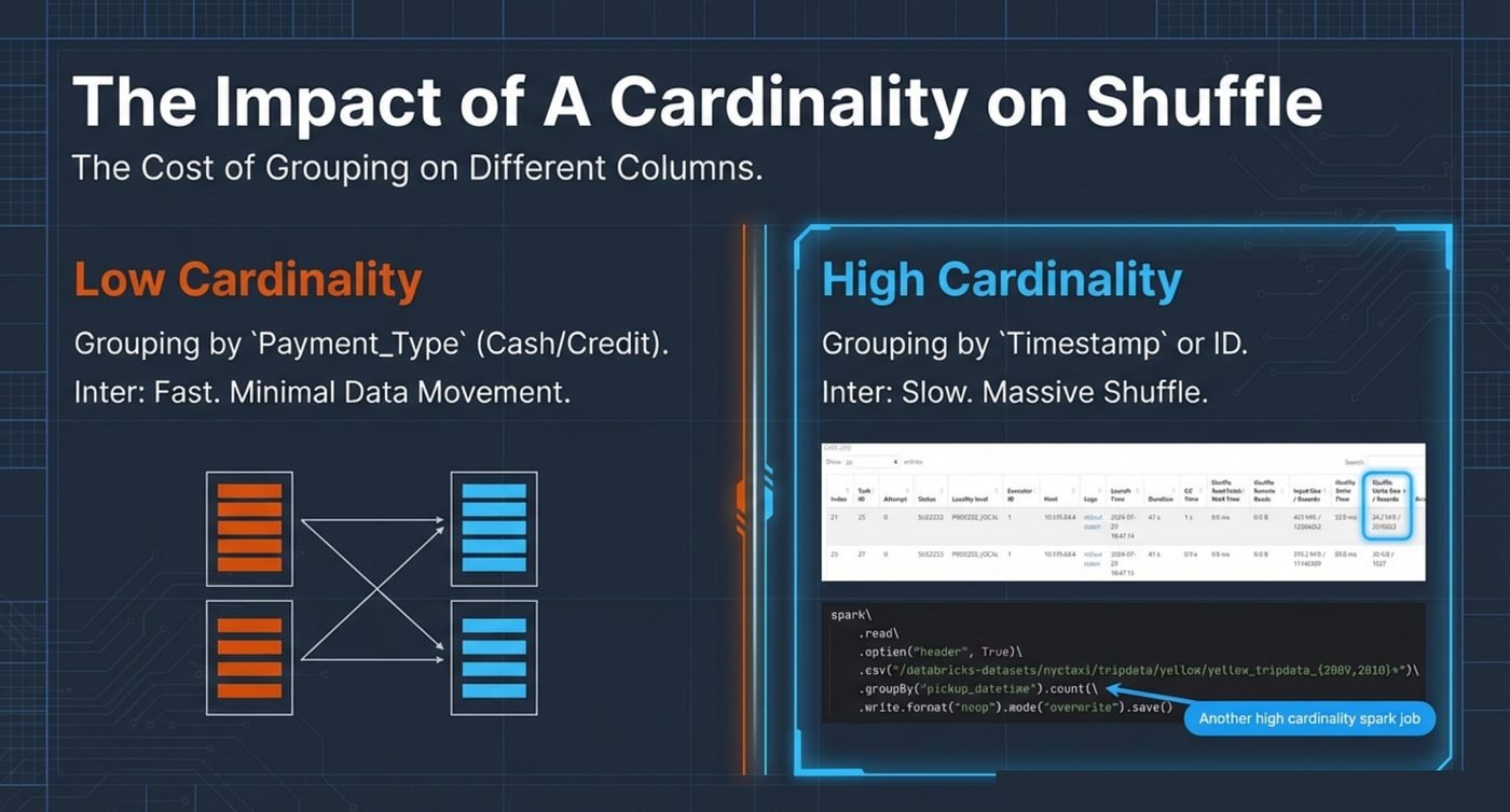
This is the one I would put in front of anyone writing their first aggregation. The cost of a groupBy is not driven by how many rows you have. It is driven by how many distinct values are in the grouping key.

Group the NYC taxi data by payment_type and you have a handful of groups. Every executor can pre-aggregate locally and send a tiny result. Group the same data by pickup_datetime and nearly every row is its own group, so there is nothing to pre-aggregate and effectively the entire dataset crosses the network.

# cheap: a few distinct values, so map side aggregation does most of the work
df.groupBy("payment_type").count()

# expensive: nearly one group per row, so the whole dataset moves
df.groupBy("pickup_datetime").count()

Same data, same line count, wildly different jobs. The shuffle write column in the task list is where you see it.

The most expensive thing you can write

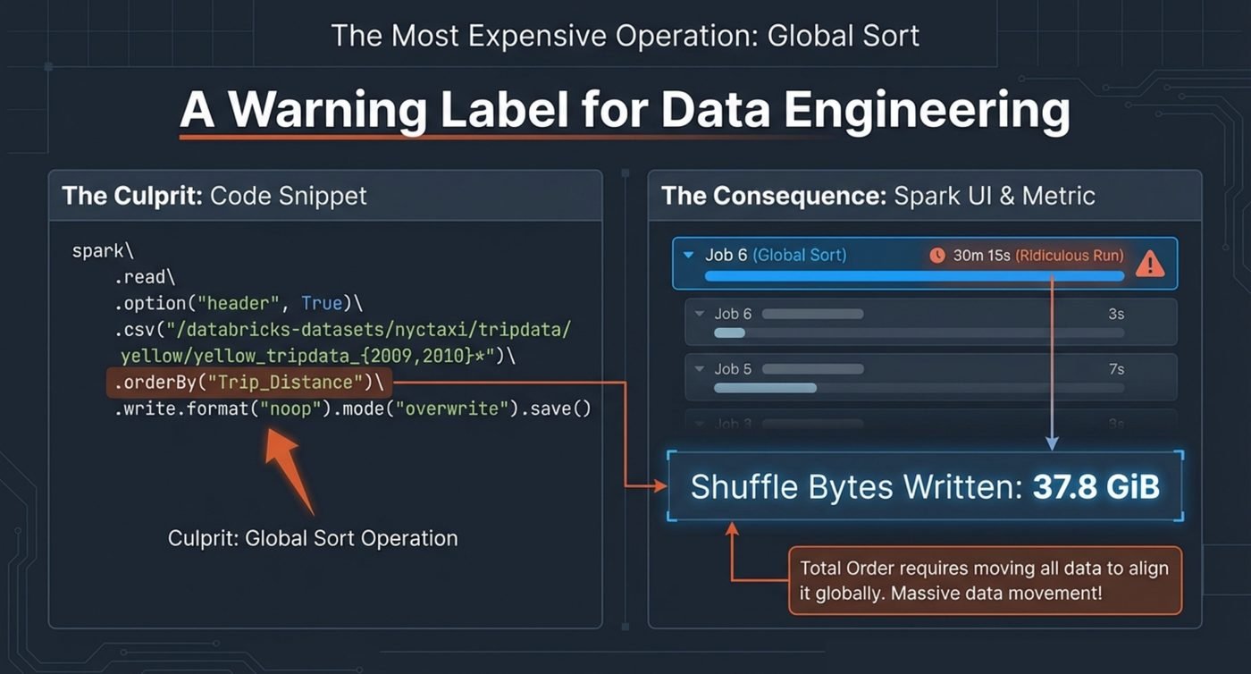
This is my favourite screenshot from the whole project, because the code looks so harmless.

spark\
  .read\
  .option("header", True)\
  .csv("/databricks-datasets/nyctaxi/tripdata/yellow/yellow_tripdata_{2009,2010}*")\
  .orderBy("Trip_Distance")\
  .write.format("noop").mode("overwrite").save()

One line. .orderBy("Trip_Distance"). And the result is 37.8 GiB of shuffle bytes written and a run of 30 minutes and 15 seconds, against neighbouring jobs finishing in three and seven seconds.

The reason is that a global sort is a total order. Every row has to be placed relative to every other row, so Spark has to sample the data to work out range boundaries, then move essentially all of it so each partition holds a contiguous range. There is no way to do that without a full redistribution.

Part four: the three optimisers

Spark has three separate optimisation systems working at different times. Knowing which one is which tells you where to look when performance is not what you expected.

Catalyst, before the job runs

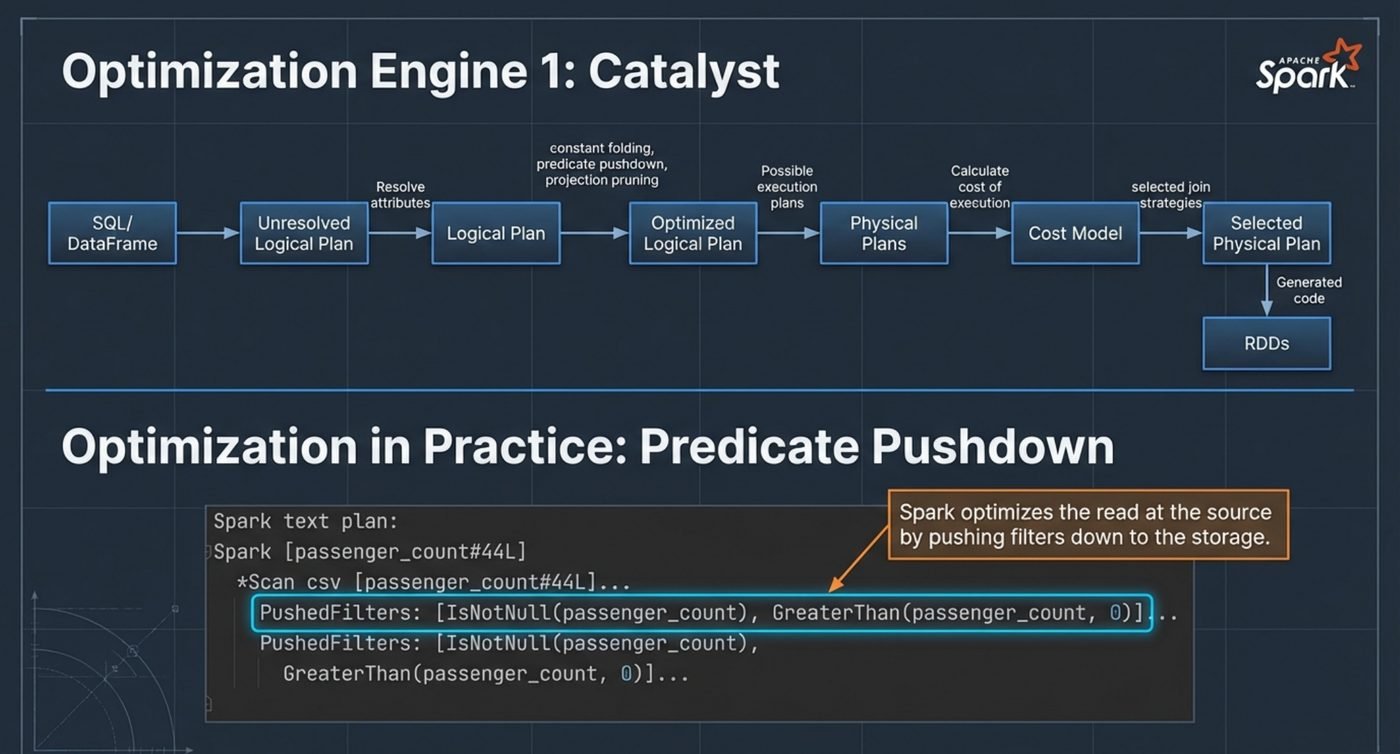
Catalyst is the rule based and cost based query optimiser. It resolves your column references, applies rewrites like constant folding, predicate pushdown and projection pruning, generates candidate physical plans, and picks one using a cost model.

The two rewrites worth knowing by name, because they are the ones your file format decides whether you get:

• Predicate pushdown pushes filters down to the scan, so the reader skips data it can prove you do not want.
• Projection pruning reads only the columns you referenced.

Both need a columnar format with statistics to work properly. On Parquet or Delta they are transformative. On CSV you get neither, because CSV has no schema, no column boundaries and no row group statistics. That is the actual reason "use Parquet" is advice rather than a preference.

Tungsten, as the code is generated

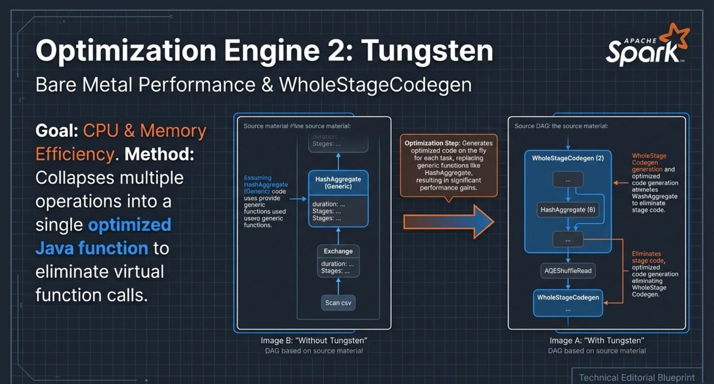
Tungsten is about CPU and memory rather than plan shape. It manages memory off heap in a compact binary format to avoid Java object overhead and garbage collection pressure, and it does whole stage code generation.

Whole stage code generation is the part you can see in the UI. Instead of running a chain of generic operators, each calling the next through a virtual function call per row, Spark generates a single Java function for the whole stage and compiles it at runtime. The boxes marked WholeStageCodegen in a DAG are stages where this happened.

This is also a diagnostic. If you see a stage that is not wrapped in WholeStageCodegen, something in it could not be fused, and a Python UDF is a very common reason.

Adaptive Query Execution, while the job runs

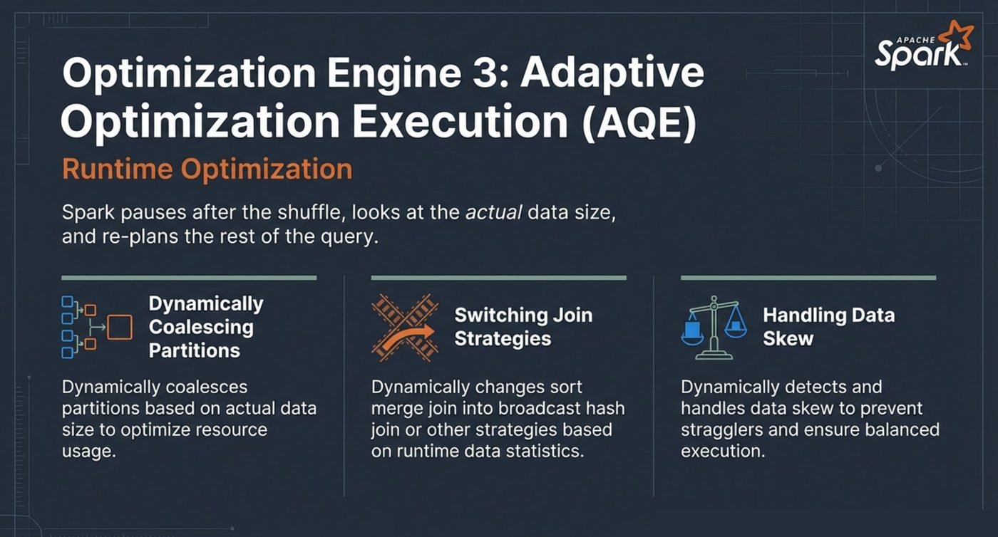
AQE is the one that changed how I think about tuning. Catalyst plans before execution using estimates, and estimates on real data are frequently wrong. AQE pauses at shuffle boundaries, looks at what actually came out, and re-plans the rest of the query with real numbers.

Three things it does:

• Coalescing partitions when the shuffle output turned out to be much smaller than expected.
• Switching join strategies, most usefully demoting a sort merge join to a broadcast hash join once it can see one side is actually small.
• Handling skew by splitting oversized partitions, so one straggler task does not hold up the whole stage.

AQE in action

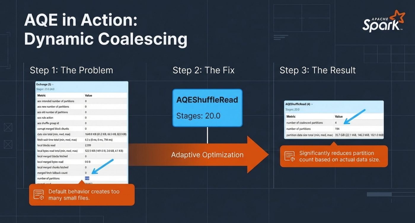
Here it is doing the first of those. The default spark.sql.shuffle.partitions is 200, and that default is applied regardless of how much data you have. On a small result you get 200 partitions, 200 tasks with scheduling overhead each, and 200 tiny output files.

The AQEShuffleRead node in the plan is AQE stepping in. In this run it took the partitions and coalesced them down to 4, based on what the shuffle actually produced.

Before AQE this was a manual chore: guess a partition count, watch it be wrong on a different day's data, add a repartition or coalesce, repeat. The small files problem in particular used to eat a lot of time. Now the honest answer for most jobs is to leave the default alone and let AQE size it, and only intervene when you can show it got it wrong.

Part five: reading the evidence

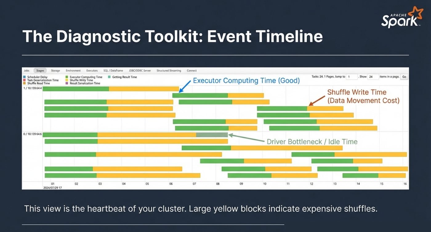
The event timeline is the view I go to first, because it answers "where did the time go" visually rather than numerically.

• Green is compute. That is the work you actually wanted.
• Yellow is shuffle read and write. That is the tax.
• Gaps are tasks not running: scheduling delay, or executors sitting idle while the driver does something.

A healthy stage is mostly green with bars that start and end together. Long yellow blocks mean you are paying for data movement, which sends you back to the shuffle questions above. Ragged bar lengths within one stage mean skew, where a few partitions are far larger than the rest, and that is what AQE skew handling is for. A wall of green followed by a long gap usually means the driver has become the bottleneck, which is often a collect() that should not be there.

Part six: who is responsible for what

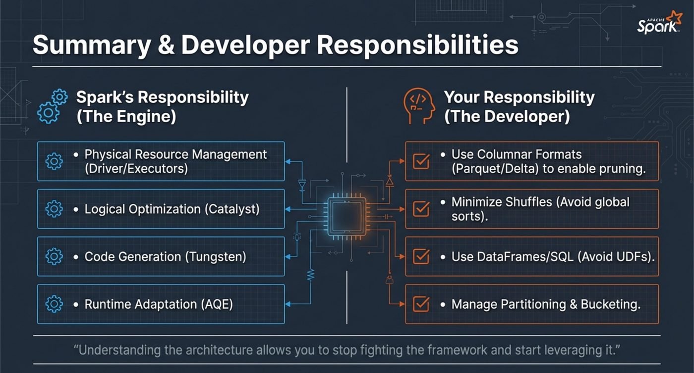
This is the slide I would keep if I could only keep one, because it draws the line honestly. Spark will do an enormous amount for you. It will not do these four things, and no amount of cluster sizing compensates for getting them wrong:

• Use columnar formats. Parquet or Delta, so pushdown and pruning have something to work with.
• Minimise shuffles. Question every wide transformation, and treat a global sort as something you have to justify.
• Use DataFrames and SQL, avoid UDFs. Keep the plan legible to Catalyst.
• Manage partitioning. Partition on something you actually filter by, and with sensible cardinality.

The quote at the bottom of that slide is the summary of the whole exercise: understanding the architecture lets you stop fighting the framework and start leveraging it.

Back to the certification

To be fair to the exam, it is not pretending to be this. It covers the Databricks platform broadly, and there is a lot of ground: the Lakehouse, Delta, Unity Catalog, jobs and orchestration, incremental ingestion. Going three levels deep on the Spark execution model would not fit, and most of the syllabus is genuinely useful.

But the questions I get asked in real work are not "which Delta command does X". They are "this pipeline takes forty minutes and it used to take eight, what changed". Answering that means reading a DAG, counting stages, spotting a shuffle that should not be there and knowing whether AQE has already dealt with it. None of that came from the certification. It came from having a slow job, a Spark UI, and enough curiosity to keep clicking.